3 Applications: Data

3.1 Case study: Passwords

Stop for a second and think about how many passwords you’ve used so far today. You’ve probably used one to unlock your phone, one to check email, and probably at least one to log on to a social media account. Made a debit purchase? You’ve probably entered a password there too.

If you’re reading this book, and particularly if you’re reading it online, chances are you have had to create a password once or twice in your life. And if you are diligent about your safety and privacy, you’ve probably chosen passwords that would be hard for others to guess, or crack.

In this case study we introduce a dataset on passwords. The goal of the case study is to walk you through what a data scientist does when they first get a hold of a dataset as well as to provide some “foreshadowing” of concepts and techniques we’ll introduce in the next few chapters on exploratory data analysis.

The passwords data can be found in the tidytuesdayR R package.

Table 3.1 shows the first ten rows from the dataset, which are the ten most common passwords. Perhaps unsurprisingly, “password” tops the list, followed by “123456.”

Table 3.1: Top ten rows of the passwords dataset.

rank	password	category	value	time_unit	offline_crack_sec	strength
1	password	password-related	6.91	years	2.170	8
2	123456	simple-alphanumeric	18.52	minutes	0.000	4
3	12345678	simple-alphanumeric	1.29	days	0.001	4
4	1234	simple-alphanumeric	11.11	seconds	0.000	4
5	qwerty	simple-alphanumeric	3.72	days	0.003	8
6	12345	simple-alphanumeric	1.85	minutes	0.000	4
7	dragon	animal	3.72	days	0.003	8
8	baseball	sport	6.91	years	2.170	4
9	football	sport	6.91	years	2.170	7
10	letmein	password-related	3.19	months	0.084	8

When you encounter a new dataset, taking a peek at the first few rows as we did in Table 3.1 is almost instinctual. It can often be helpful to look at the last few rows of the data as well to get a sense of the size of the data as well as potentially discover any characteristics that may not be apparent in the top few rows. Table 3.2 shows the bottom ten rows of the passwords dataset, which reveals that we are looking at a dataset of 500 passwords.

Table 3.2: Bottom ten rows of the passwords dataset.

rank	password	category	value	time_unit	offline_crack_sec	strength
491	natasha	name	3.19	months	0.084	7
492	sniper	cool-macho	3.72	days	0.003	8
493	chance	name	3.72	days	0.003	7
494	genesis	nerdy-pop	3.19	months	0.084	7
495	hotrod	cool-macho	3.72	days	0.003	7
496	reddog	cool-macho	3.72	days	0.003	6
497	alexande	name	6.91	years	2.170	9
498	college	nerdy-pop	3.19	months	0.084	7
499	jester	name	3.72	days	0.003	7
500	passw0rd	password-related	92.27	years	29.020	28

At this stage it’s also useful to think about how these data were collected, as that will inform the scope of any inference you can make based on your analysis of the data.

Do these data come from an observational study or an experiment?³⁹

There are 500 rows and 7 columns in the dataset. What does each row and each column represent?⁴⁰

Once you’ve identified the rows and columns, it’s useful to review the data dictionary to learn about what each column in the dataset represents. This is provided in Table 3.3.

Table 3.3: Variables and their descriptions for the passwords dataset.

Variable	Description
rank	Popularity in the database of released passwords.
password	Actual text of the password.
category	Category password falls into.
value	Time to crack by online guessing.
time_unit	Time unit to match with value.
offline_crack_sec	Time to crack offline in seconds.
strength	Strength of password, relative only to passwords in this dataset. Lower values indicate weaker passwords.

We now have a better sense of what each column represents, but we do not yet know much about the characteristics of each of the variables.

Determine whether each variable in the passwords dataset is numerical or categorical. For numerical variables, further classify them as continuous or discrete. For categorical variables, determine if the variable is ordinal.

---

The numerical variables in the dataset are rank (discrete), value (continuous), and offline_crack_sec (continuous). The categorical variables are password, time_unit. The strength variable is trickier to classify – we can think of it as discrete numerical or as an ordinal variable as it takes on numerical values, however it’s used to categorize the passwords on an ordinal scale. One way of approaching this is thinking about whether the values the variable takes vary linearly, e.g., is the difference in strength between passwords with strength levels 8 and 9 the same as the difference with those with strength levels 9 and 10. If this is not necessarily the case, we would classify the variable as ordinal. Determining the classification of this variable requires understanding of how strength values were determined, which is a very typical workflow for working with data. Sometimes the data dictionary (presented in Table 3.3) isn’t sufficient, and we need to go back to the data source and try to understand the data better before we can proceed with the analysis meaningfully.

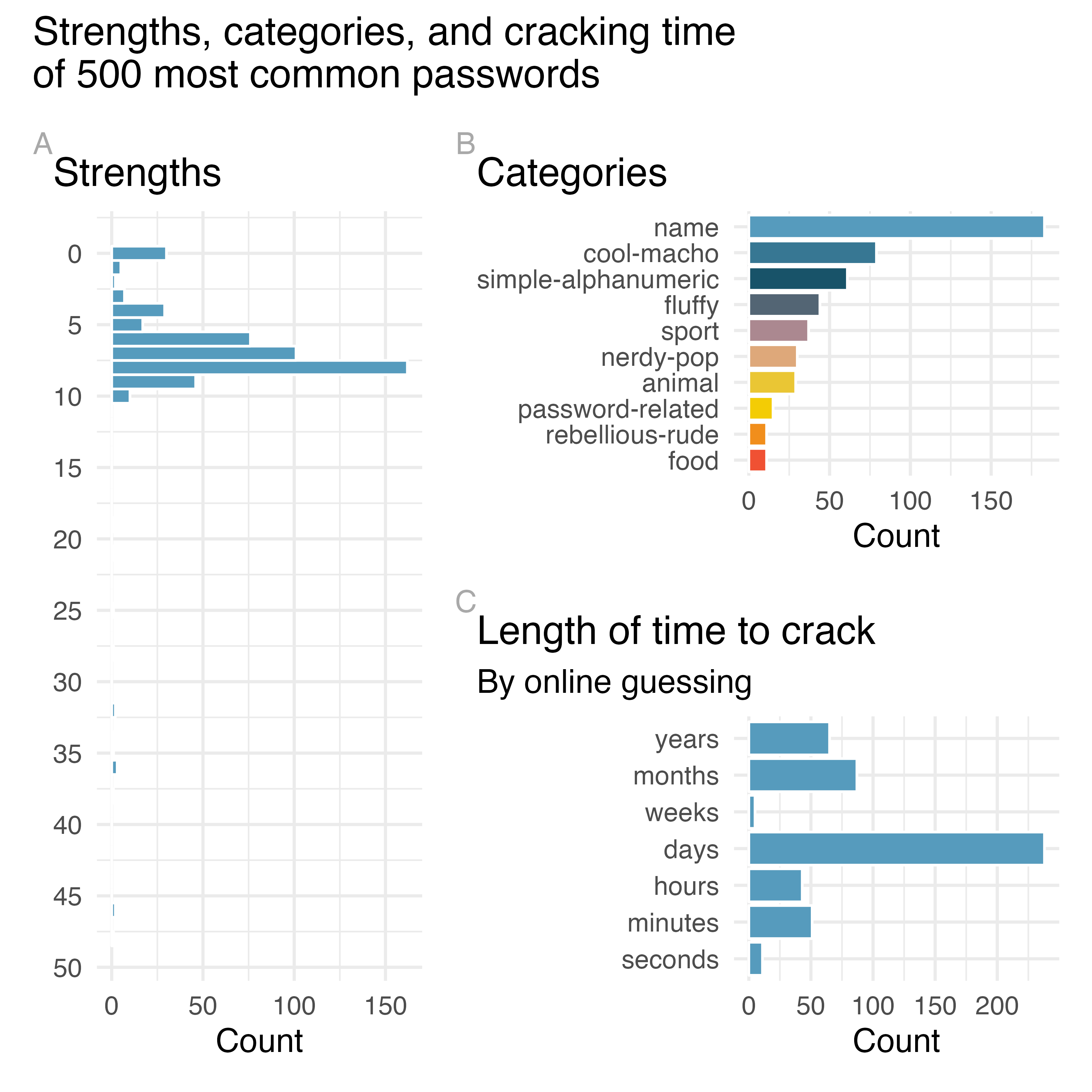
Next, let’s try to get to know each variable a little bit better. For categorical variables, this involves figuring out what their levels are and how commonly represented they are in the data. Figure 3.1 shows the distributions of the categorical variables in this dataset. We can see that password strengths of 0-10 are more common than higher values. The most common password category is name (e.g. michael, jennifer, jordan, etc.) and the least common is food (e.g., pepper, cheese, coffee, etc.). Many passwords can be cracked in the matter of days by online cracking with some taking as little as seconds and some as long as years to break. Each of these visualizations is a bar plot, which you will learn more about in Chapter 4.

Figure 3.1: Distributions of the categorical variables in the passwords dataset. Plot A shows the distribution of password strengths, Plot B password categories, and Plot C length of time it takes to crack the passwords by online guessing.

Similarly, we can examine the distributions of the numerical variables as well. We already know that rank ranges between 1 and 500 in this dataset, based on Table 3.1 and Table 3.2. The value variable is slightly more complicated to consider since the numerical values in that column are meaningless without the time unit that accompanies them. Table 3.4 shows the minimum and maximum amount of time it takes to crack a password by online guessing. For example, there are 11 passwords in the dataset that can be broken in a matter of seconds, and each of them take 11.11 seconds to break, since the minimum and the maximum of observations in this group are exactly equal to this value. And there are 65 passwords that take years to break, ranging from 2.56 years to 92.27 years.

Table 3.4: Minimum and maximum amount of time it takes to crack a password by online guessing as well as the number of observations that fall into each time unit category.

time_unit	n	min	max
seconds	11	11.11	11.11
minutes	51	1.85	18.52
hours	43	3.09	17.28
days	238	1.29	3.72
weeks	5	1.84	3.70
months	87	3.19	3.19
years	65	2.56	92.27

Even though passwords that take a large number of years to crack can seem like good options (see Table 3.5 for a list of them), now that you’ve seen them here (and the fact that they are in a dataset of 500 most common passwords), you should not use them as secure passwords!

Table 3.5: Passwords that take the longest amount of time to crack by online guessing.

rank	password	category	value	time_unit	offline_crack_sec	strength
26	trustno1	simple-alphanumeric	92.3	years	29.0	25
336	rush2112	nerdy-pop	92.3	years	29.0	48
406	jordan23	sport	92.3	years	29.3	34
500	passw0rd	password-related	92.3	years	29.0	28

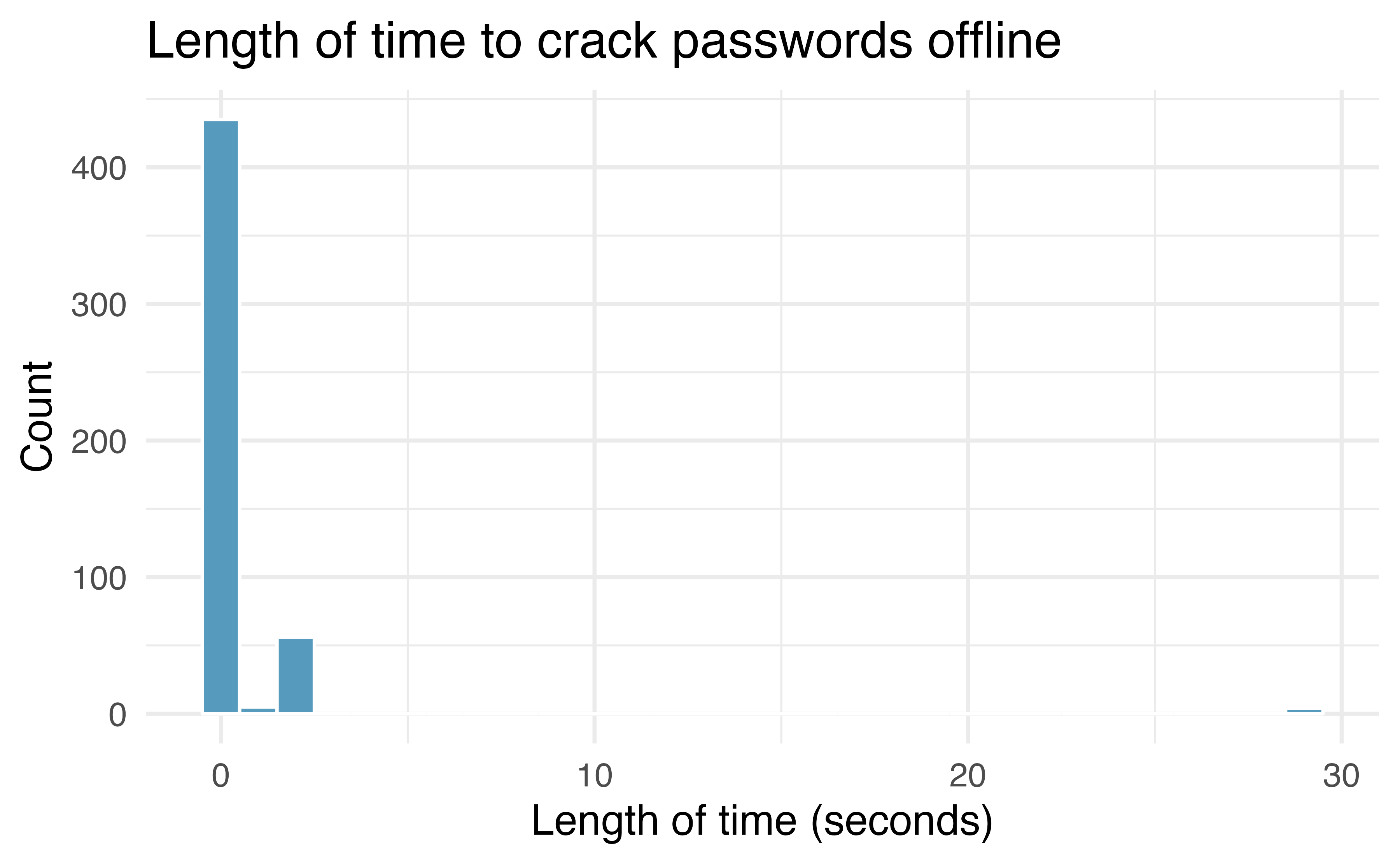
The last numerical variable in the dataset is offline_crack_sec. Figure 3.2 shows the distribution of this variable, which reveals that all of these passwords can be cracked offline in under 30 seconds, with a large number of them being crackable in just a few seconds.

Figure 3.2: Histogram of the length of time it takes to crack passwords offline.

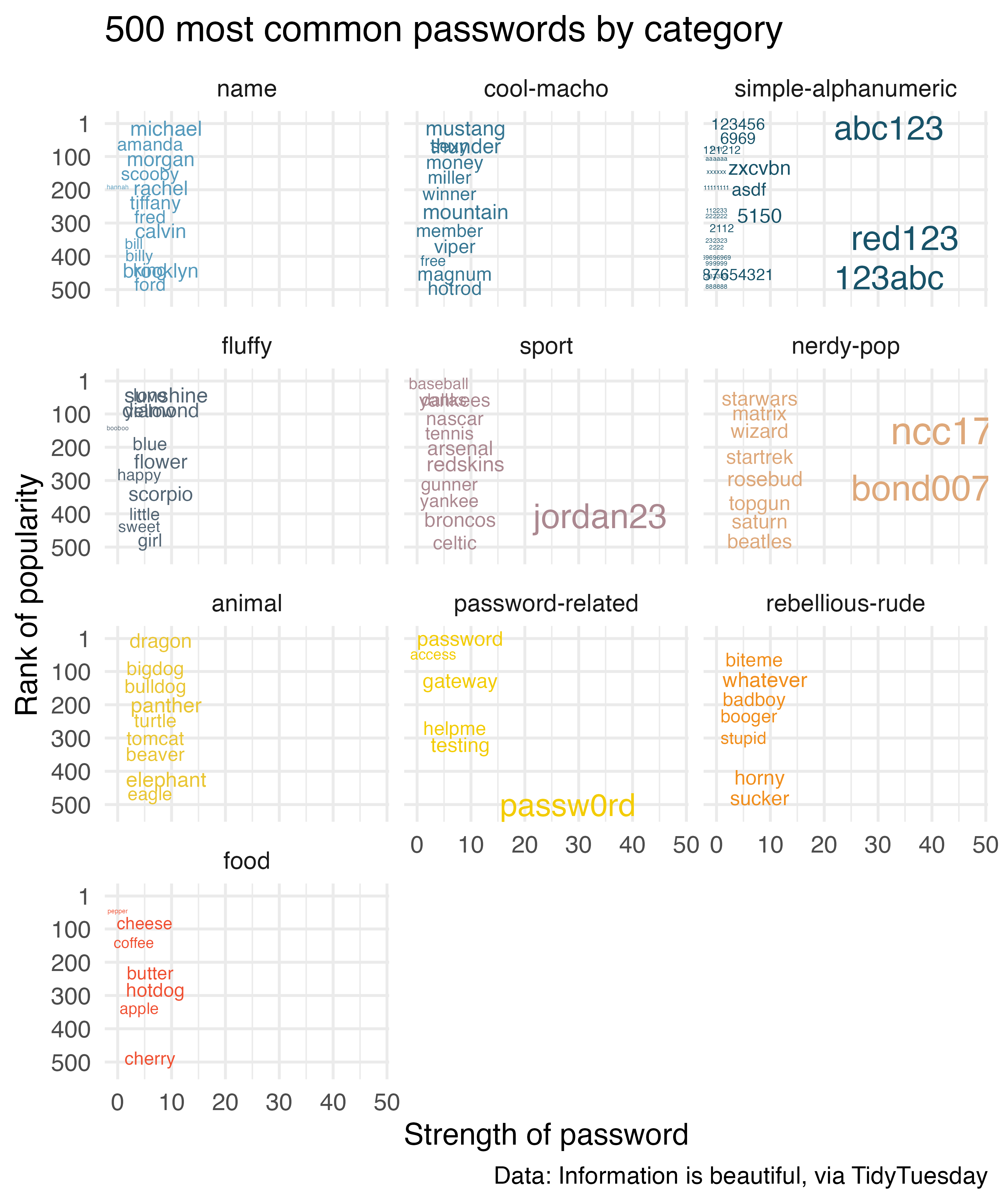
So far we examined the distributions of each individual variable, but it would be more interesting to explore relationships between multiple variables. Figure 3.3 shows the relationship between rank and strength of passwords by category, where more common passwords (those with higher rank) are plotted higher on the y-axis than those that are less common in this dataset. The stronger the password, the larger text it’s represented with on the plot. While this visualization reveals some passwords that are less common, and stronger than others, we should reiterate that you should not use any of these passwords. And if you already do, it’s time to go change it!

Figure 3.3: Rank vs. strength of 500 most common passwords by category.

In this case study, we introduced you to the very first steps a data scientist takes when they start working with a new dataset. In the next few chapters, we will introduce exploratory data analysis and you’ll learn more about the various types of data visualizations and summary statistics you can make to get to know your data better.

Before you move on, we encourage you to think about whether the following questions can be answered with this dataset, and if yes, how you might go about answering them. It’s okay if your answer is “I’m not sure,” we simply want to get your exploratory juices flowing to prime you for what’s to come!

1. What characteristics are associated with a strong vs. a weak password?
2. Do more popular passwords take shorter or longer to crack compared to less popular passwords?
3. Are passwords that start with letters or numbers more common among the list of top 500 most common passwords?

3.2 Interactive R tutorials

Navigate the concepts you’ve learned in this chapter in R using the following self-paced tutorials. All you need is your browser to get started!

Tutorial 1: Introduction to data

Tutorial 1 - Lesson 1: Language of data

Tutorial 1 - Lesson 2: Types of studies

Tutorial 1 - Lesson 3: Sampling strategies and experimental design

Tutorial 1 - Lesson 4: Case study

You can also access the full list of tutorials supporting this book here.

3.3 R labs

Further apply the concepts you’ve learned in this part in R with computational labs that walk you through a data analysis case study.

Intro to R - Birth rates

You can also access the full list of labs supporting this book here.